

INTRODUCTION TO PROBABILITY
Lecture 37. Application to Markov processes. The Wiener
process.
Theorem 37.1. Let  be a probability measure on the space (X,
  ),
and let
),
and let
P( s, x, t, C) be a function of the times s, t, 0≤ s≤t, of x ∈X, and of a set C
∈
,
such that for fixed s, t; and x it is a probability measure as a function of C;
for fixed
s, t, and C it is measurable as a function of x; P (t, x, t, C) =  (C);
and this function
(C);
and this function
satisfies the Chapman - Kolmogorov equation:
Then the finite-dimensional distributions  defined, for 0 ≤ t1≤ t2 ... ≤tn,
by
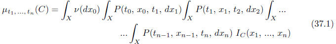
satisfy the consistency conditions.
The proof is very simple: it could seem that the conditions imposed on P
(s, x, t, C)
were designed specially so that the proof is easy. The condition (36.9n+1)
is satisfied
because P (tn, xn, tn+1, X) = 1, and conditions
(9i), 1 ≤ i ≤ n, because of the Chapman {
Kolmogorov equality
So if the space (X, ![]() )
is not extremely ugly (e. g. a non-Borel set with I don't
)
is not extremely ugly (e. g. a non-Borel set with I don't
know what as the σ-algebra in it), there exists a stochastic process with the
prescribed
finite-dimensional distributions, and by Theorem 34.1 it is a Markov process
with initial
distribution ν and transition function P( , , ,). In particular, there is
a Markov
process corresponding to the transition function you invented solving Problem 54
. Can
you say anything about this Markov process of yours; apart from its
finite-dimensional
distributions?
Another example:
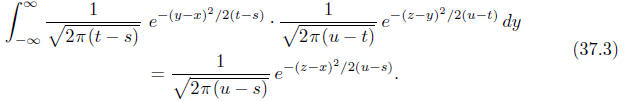
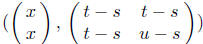
Example 37.1. Take 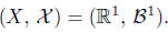 The transition
density
The transition
density

(as a function of y, it is the density of the normal distribution with
parameters (x, t-s))
satisfies the Chapman -Kolmogorov equation:
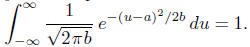
One of the ways to check it is to collect all terms with y2,
with y, and with no
y in the quadratic function being the exponent in the integrand, and use the
fact that
Another way: For fixed x, the integrand in (37.3) is, as a
function of y, z, the den-
sity of the two-dimensional normal distribution with parameters
(check it!); the integral with respect to y, as a function of z, represents the
density of the
second coordinate: that of the normal distribution with parameters (x, u- s).
A third way: the left-hand side integral in (37.3) is the convolution formula
for the
probability density of the sum of two independent one-dimensional random
variables 
and  , where
has the normal distribution with parameters
(x, t - s), and the second,
, where
has the normal distribution with parameters
(x, t - s), and the second,
, with parameters (0, u- t). The characteristic function
 of the
sum is equal to the product of their characteristic functions:

 the characteristic function corresponding to
the normal density in the right-hand side of (37.3) (you see, I am running out
of letters).
Problem A Check that the density
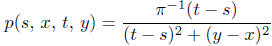 satisfies the
Chapman -Kolmogorov equation.
A stochastic process is a function  of two
arguments: the "time"
of two
arguments: the "time" 
and the sample point ω∈Ω.
If we fix t ∈ T, the function  of the second
argument is a random variable.
of the second
argument is a random variable.
If we fix ω, is just a function of "time". We
call this function a trajectory (a
is just a function of "time". We
call this function a trajectory (a
sample function) of our stochastic process.
A stochastic process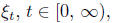 with values in
 is called a Wiener process
if its finite-dimensional distributions![]() are given by formula (37.1) with
are given by formula (37.1) with
and all its trajectories are continuous:
![]() is continuous in t
for every ω∈Ω
is continuous in t
for every ω∈Ω
We have proved that it is possible to satisfy the first part of the definition {
that
about the finite-dimensional distributions; but we know nothing about the second
part {
about all trajectories being continuous. The credit for this belongs to N.Wiener.
The Wiener process is the mathematical model for the physical phenomenon of
Brownian motion:
the process of motion of a light particle in a fluid under the influence of
chaotic impulses from molecules
hitting it. That is, the Brownian motion is three-dimensional (or
two-dimensional if we want to model what
we see under the microscope), while we consider the one-dimensional Wiener
process; more accurate would
be saying that the Wiener process is the mathematical model of one coordinate of
the physical Brownian
motion.
The stochastic process![]() having the given finite-dimensional distributions
having the given finite-dimensional distributions
(no matter what these distributions are) constructed in the proof of
Kolmogorov's Theorem
(Theorem 35.2) clearly doesn't have all trajectories
continuous: the trajectories
![]() =
=
 are all functions belonging to
 (all real-valued functions on the interval
[0, 1)), and we know that there are discontinuous functions. We cannot state
either that
almost all functions  are continuous: it can
be proved easily that
are continuous: it can
be proved easily that 
makes no sense: the set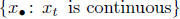 does not belong to
the
does not belong to
the 
We may hope that there is, on the same probability space
 , another
stochastic process![]() , t
∈ [0, ∞), with the same finite-dimensional distributions, but with
, t
∈ [0, ∞), with the same finite-dimensional distributions, but with
continuous trajectories.
Theorem 37.2. If  and
and
 are two random functions; and
 for every t ∈ T, then the random functions
 and
and
 have the same
finite-dimensional distributions.
Proof. We have to prove that for every natural n, for every t1,
..., tn ∈ T, and for
every C∈ 

The symmetric difference of the events and
and  is
is
clearly a subset of the event and the
probability of this union
and the
probability of this union
is not greater than
In the next lecture we'll have a bigger theorem that will help us to prove the
existence
of a Wiener process.