REVIEW OF MATH

2.2 Multivariate calculus refresher

The part of these notes addressed functions where a single input goes in, and a single
output comes out. Most economic applications aren’t so simple. In most cases, a
number of variables influence a decision, or a number of factors are required to
produce some good. These are functions of many variables. If the variable z is a
function of x and y, this is written:

z = f (x, y)

Of course, f could be a function of more than two inputs. A production function
might have capital, labor, and material inputs:

Y = F(K, L,M)

Utility might be a function of goods:

Demand for a particular good   is a function of the price of that good, the price of
another good , and the person’s wealth:

In previous micro classes, you discussed about how quantity demanded changes
when something else, like the price of , changes, “holding everything else constant”
or ceteris paribus. This translates into the idea of a partial derivative, denoted by:

The price of good x is held constant, and wealth is held constant—though the
person’s wealth may change if he is a large producer of good y, we’re not concerned
about those possible effects. Similarly, we might talk about the marginal product of
labor (denoted by or simply ), and the marginal utility of
consuming good (denoted by ).

Taking a partial derivative is like pretending f (x, y) is just a function of x,
with y constant. Because of this, the addition rule, the product rule, and the
quotient rule work the same as in the univariate case.

Considering that other factors may change is the notion of a total derivative.
Using the previous example, consider that demand for x is a composite function of
prices and wealth, which is itself a function of prices:

Then the total derivative of x with respect to the price of y is:

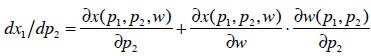
The first term on the right-hand side is the partial derivative of x with respect to
price of y. This tells you the effect holding everything else constant. For the total
derivative, we also add in these other effects—in this case, that the person’s wealth
changes when the price of y changes, and that his demand for x changes when his
wealth changes. The second term on the right-hand side comes from applying the
chain rule. Intuitively, the partial derivative captures the substitution effect
of a price change, while the total derivative contains both the substitution
and income effects.

Similar to derivatives are differentials. Remember that, given a change in the run
of a function (back to one variable) you can use the slope at that point to
approximate the change in the rise:

When the Δx get really, really tiny this is a good approximation. When they get
infinitely tiny or infinitesimal,  this turns out to be exactly correct, not an
approximation at all. The convention in calculus is, of course, to use dx to denote
this small change:

This is known as a differential. If you divide both sides by dx, you get the derivative.
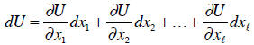
In multivariate calculus, a function and its differential might look like:

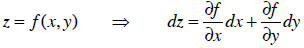
The way that I figure out differentials is by writing down a list of all the variables
(dependent or independent) and then going through the function. Whenever a term
shows up that has one of these variables, I take the partial derivative of that term
and I tack on a dx or whatever the variable is. If the term has multiple variables in it,
I do this for each of them. Consider the relationship:

The differential of this function is:

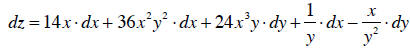
If we say y doesn’t change, and we want to see what the effect of a small change in x
on z is, we set dy = 0 . Not surprisingly, the result is exactly the same as the partial
derivative of z with respect to x. Additionally, we might be interested in changing
both x and y a small bit, and see the result on z. We can also do this using the
differential.

Differentials are more versatile than just taking the derivative. Let’s say we have the
production function:

Y = F(K, L, M)

where capital, labor, and materials are our inputs. The differential of this production
function is:

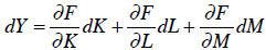
That equation says that the change in output depends on the change in capital and
the marginal product of capital, the change in labor times the marginal product of
labor, and the change in materials times the marginal product of materials. That’s a
true, indisputable fact.

We can use that fact in the following manner. Suppose we want to keep output the
same, and see how much less of one factor (capital) we would need if we reduce
another (labor) from the same materials. In other words, we want to keep dY = 0
and dM = 0 , and we need to find the values of dK and dL that balance the equation:

With some rearranging, this produces the following result:

This is change in capital necessary to keep production the same. In economics, it is
interpreted as the marginal rate of technical substitution. If you remembered
from previous classes that the MRTS of labor for capital is the ratio of their marginal
products, you’ve now seen where that result comes from. What we have found here
is the slope of the isoquant curve at a particular point.

Another interesting question would is how much of one good a person would require
to offset in utility changes from a change in another good. Let’s say there are l
goods, labeled through , in the person’s utility function:

The differential of this function is:

We want to know how much of good k the person would trade for good m, keeping
his utility the same. He is not trading another other goods. Then:

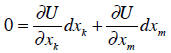
Rearranging produces the marginal rate of substitution:

Again, you may recall that the MRS equals the ratio of marginal utilities. It should
also be the slope of a line tangent to the indifference curve at that point. Think
about this in a two-good world—draw some pictures in space. If we start
with a particular point and name all others points which do not change the utility—
that is, the set of all points such that dU=0—we’ve identified an indifference curve.
Its slope at this particular point would be described by , which is exactly
what we found here.

Indifference curves and technology frontiers are both examples of implicit
functions. An explicit function is what we usually think of as a function:

y = f (x)

An implicit function looks like:

c = f (x, y)

where c is some constant (or at least a constant, as far as we’re concerned). Think
about indifference curves and isoquant curves, which show the values of x and y that
yield the same utility or output c: these are implicit functions.

Sometimes we get a relationship between x and y that’s virtually impossible to solve
for one in terms of the other. For instance, try solving this for y:

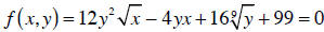
Given that you can’t isolate y, is there any hope of figuring out dy/dx ? Yes, using the
differential as before:

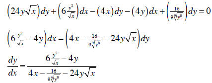
The point is that even if you can’t solve y explicitly in terms of x, you can still
evaluate its derivative.

More importantly, often you don’t even know the exact function (because you’re
working with an arbitrary U(x, y) ), which makes it impossible to solve explicitly for
one variable in terms of another. You can still look at marginal effects, as we did
earlier. These are all applications of my favorite principle in mathematics, the
implicit function theorem.

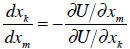
Theorem: Let f (x, y) = c implicitly define y as a function of x, for some constant c. Then
the derivative of y with respect to x is

This is very useful in economics. For instance, consider a person who gets utility
from consumption of two goods, x and y. We’ll set the price of the first good to 1,
and let p be the price of the second. The budget constraint requires
that y = (w - x) /p . Substituting this into the utility function, we have that:

The utility function is:

U(x, y) =U(x, (w - x) /p)

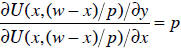
We usually find that a utility maximizing individual sets the marginal rate of
substitution between the goods equal to the relative prices:

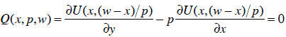
How does a change in the price (or wealth) affect consumption of x? One side of the
equation needs to be a constant, which can almost always be achieved by simply
subtracting one side off. It also looks like we can make things simpler by multiplying
through by the denominator. Let’s give this implicit function the name Q:

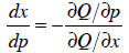
The implicit function theorem tells how to find all of these effects; for example, we
can use this function to determine how demand changes when prices change:

The neat thing about this is it gives us an answer that depends on diminishing
marginal utilities of the goods (second derivatives) as well as their complementarity
or substitutability (cross-partial derivatives)—and we’ve assumed nothing about the
utility function.